For a general introduction to credit risk, please review Part 1.
Quantitative measurements of Credit Risk and Credit Value at Risk (CVaR) model
The key point in terms of credit risk evaluation is the calculation of expected loss. The one-year expected loss for a single loan corresponds to the mathematical product of the one-year probability of default, the loss given default rate, and the exposure at default amount presented by the formula below:
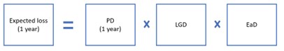
Probability of default (PD) – measures the likelihood of the obligor defaulting on the terms of a contract.
Loss given default (LGD) – represents the likely percentage loss if the borrower defaults.
Exposure at default (EaD) – is the total value the creditor is exposed to when a default event occurs.
Probability of default is an important component for the calculation of the expected loss. At FS Impact Finance, we use a model known as the Ratings Transition matrix (a.k.a. Ratings Migration matrix) for Credit Value at Risk (CVaR) calculations. The Rating Migration matrix is based on the individual ratings assigned to separate obligors and it captures the rating migration probabilities over a given time horizon. In other words, it provides the probabilities for whether the rating will remain the same, upgrade or downgrade, or even jump immediately to default status.
The migration matrix is used to assess the portfolio risk due to changes in debt value caused by changes in the obligor’s credit quality. Here we are dealing with the so-called credit migration risk, which describes the risk of potential loss due to changes in credit quality and resulting changes of credit ratings. Credit migration risk analysis is a fundamental technique in CVaR models.
In the sample transition matrix demonstrated below, the probability that a borrower rated AAA at the start of a period will have a rating of BBB+ at the end of the period would be 0,01 %, as shown in the first row of the table:
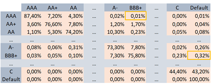
The probability of default for one year can be inferred from the last column of the rating transition matrix. In the table above, the one-year PD for a loan with a rating grade of BBB+ is 0,32 % and the one-year PD for a loan with rating grade of C is 43,2 %. As one would expect, the default probabilities are increasing as the ratings become worse, and finally for a rating D (default), 100 % probability of default is assigned.
Credit Value at Risk (CVaR)
CVaR is a popular method for measuring credit risk of the loan portfolio. In general, value at risk models quantify the extent of possible financial losses within a firm, portfolio, or position and are associated with the concepts of time horizon and confidence level. The time horizon is the specific time frame over which the model is quantifying the loss, e.g. it can be 1 year. The confidence level is the probability that the value of a parameter falls within a specified range of values. The goal is to estimate the loss level that is going to occur in a small fraction of the cases.
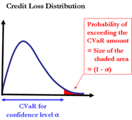
When we say, “For a confidence level of 99 % and a time horizon of 1 year, the portfolio’s CVaR figure equals to EUR 100,000”, this means that “It is 99 % certain that over a period of 1 year, credit losses in the portfolio will not exceed EUR 100,000”. Also, we could say, “The likelihood that credit losses over 1 year will exceed EUR 100,000 is only 1.0 %”. In the graphical presentation below, we can see that for the given credit loss distribution, the probability of exceeding the CVaR amount equals the size of the shaded area.
Unless unduly restrictive assumptions are used, CVaR cannot be calculated analytically but should be approximated using either Monte Carlo simulation or an analytical approximation. In the context of FS Impact Finance CVaR application, the “Conditional Moment Matching” approach due to Puzanova et al. (2009) is applied. The theoretical foundation of model in use is Vasicek’s (2002) adaptation of Merton’s (1974) approach to the pricing of corporate debt.
The two approaches broadly distinguished in the financial literature within the context of CVaR calculation, namely, the more complex Monte Carlo simulation and the more straightforward parametric approach, are briefly discussed below. When either one is applied, we should bear in mind the limitations and shortcomings of the respective model.
The Monte Carlo simulation
The Monte Carlo1 simulation method of CVaR calculation aims to find the loss level corresponding to the confidence level of 99.9 % via generating the loss distribution by direct Monte-Carlo simulations.
The Monte-Carlo simulation is generated in several steps as described below.
- First, defaults and losses over each obligor of the portfolio are estimated. This consists of assigning a rating and a loss given default to each obligor.
- Then the dependence between obligors is estimated. In practice, either pairwise asset correlations are determined, or obligors are assigned an industry sector and a country, and industry and country correlations are then defined.
- In the next step, the correlated defaults and loss given defaults are calculated, taking into account any securities, like guarantees and collaterals, to consider the real losses.
- Then the losses are computed at the transaction level and added up at the portfolio level.
- By repeating the above steps many times, the loss distribution and the relevant indicators are computed.
The Monte-Carlo simulation is a quite complex process and requires specially designed software. When using this methodology, one should always keep in mind that the results are only statistical estimates and not exact figures. Errors are possible due to its complexity, how the inputs are gathered and processed, the underlying assumptions, etc.
The Parametric CVaR
The parametric CVaR approach assumes that economic capital is a multiple of the standard deviation of the credit losses. The parametric CvaR depends on the standard deviation of the loss on each line of the portfolio and on the correlations between each line.
Below is a generic formula which represents this approach:
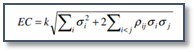
Where
σi is the unitary standard deviation of line i of the portfolio.
ρij is the loss corelation between line i and line j of the portfolio.
k is a coefficient called the capital multiplier which is calibrated in order to be consistent with the 99.9 % threshold.
The main advantage of this approach is that it leads straightforwardly to estimate of the marginal contribution and incremental capital of any line of the portfolio.
Conclusion – part 2
Throughout the evolution of credit risk modelling, different approaches have been developed in order to quantify credit risk and arrive at a reasonable interpretation for its measurement. One of the popular approaches for credit risk quantification is the CVaR model which aims to capture the downside value of a credit portfolio.
There is no single best approach agreed in financial literature in terms of risk management practices and quantitative models applied. Nonetheless, the best practices developed so far can serve as a great resource for financial institutions to elaborate their own internal methodologies and risk management practices in line with their national standards and regulations.
And when thinking of the resources needed to develop a strong and sound risk management framework, it might be a good idea to keep in mind an old saying, “An ounce of prevention is worth a pound of cure”.
Footnotes
1 The name Monte Carlo refers to the casino-laden neighbourhood of Monaco. The authors referred to how much chance applies. Isn’t it noteworthy that a complex statistical model can be approximated to a game of roulette?